Basic Forest Inventory with UAV Structure from Motion
This post outlines how to identify and measure trees from 3d point cloud data. The point cloud was created using the structure from motion (SfM) process from images collected using a fixed-wing unmanned aerial vehicle (UAV). Sparing you the many details on SfM, UAVs, and how cool these new technologies are, I wanted to show you how to do some simple and fun analysis on drone data. First off, let’s load the SfM point cloud (file is provided for you in ‘data’ directory), then we can plot it and have a look at the raw point cloud. It shows a few ponderosa pine (Pinus ponderosa) trees in the vast sea of ponderosa pine forest in northern Arizona.
pacman::p_load("rLiDAR","lidR","raster","rgdal","dplyr")

las.raw <- lidR::readLAS("sfm_pointcloud.las")
Before we get started, we need to get the point cloud set up correctly so we can treat it like a regular lidar-based point cloud. First, assign the point return values with ‘1’ to prevent processing issues (a SfM point cloud doesn’t technically have a return number since the points are image-derived). Then. assign the point cloud a reference coordinate system, the data for this example are located in UTM Zone 12N (outside of Flagstaff, AZ, USA). Now we can separate (i.e. classify) the ground and non-ground points from one another using the ‘Cloth Simulation Filter’ method. This enables smoother tree identification later on. Let’s take a look at how the classification did, notice that the non-ground points are mostly trees and some debris on the ground surface (rocks, understory vegetation, etc.). Overall it looks pretty good.
las.raw@data$ReturnNumber[las.raw@data$ReturnNumber == 0] <- 1

crs(las.raw) <- "+init=epsg:32612"

mycsf <- csf(sloop_smooth = TRUE, class_threshold = 1.37, cloth_resolution = 1, rigidness = 2)

las.raw <- lasground(las.raw, mycsf)

# I comment this line out because 3d plotting isn't supported here. But here's what mine looks like.
#plot(las.raw, color="Classification")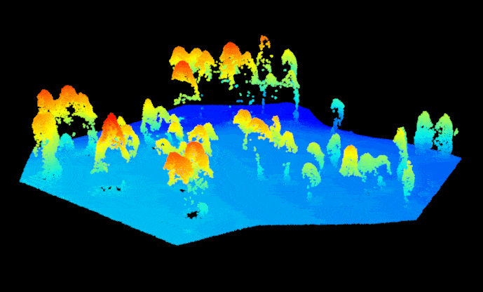
Now, let’s make a digital terrain model (DTM). The DTM provides an unobstructed ground surface, which we later use to ‘normalize’ the points in the point cloud. This almost literally puts all points on a level playing field, ensuring that a point’s height off the ground can be compared across the entire point cloud. I have found a good set of parameters to create the DTM using the KKN/IDW method with the grid_terrain() function in the lidR package, results can vary depending on your data.
dtm <- lidR::grid_terrain(las.raw, algorithm = knnidw(k = 11, p = 2))

crs(dtm) <- "+init=epsg:32612"

plot(dtm, main = "Digital Terrain Model (DTM)", legend.args = list(text = 'Elevation (m)'))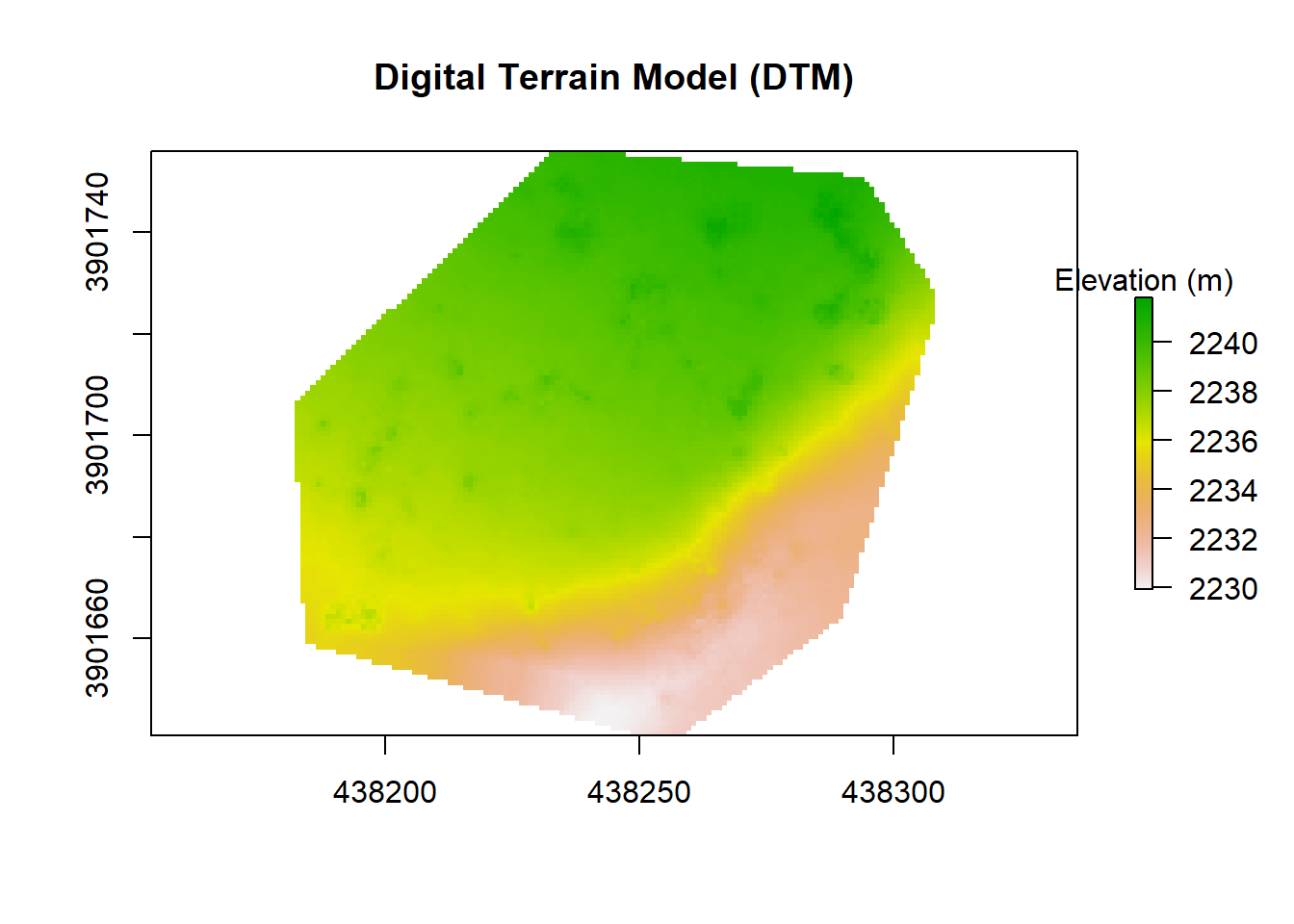
Now we can normalize the point cloud using the DTM. After it’s normalized, we assign values of points with height values less than 0 to be 0. This ensures that any below ground ‘noise’ doesn’t get incorporated into the final result. Below ground noise is common in SfM point clouds where the ground isn’t always visible and other quality issues arise. Since the method we are using to perform the individual tree segementation (Li et al., 2012) doesn’t require using a canopy height model, we are just making this to help visualize the data (and for fun!).
las.norm <- lasnormalize(las.raw, dtm)

las.norm@data$Z[las.norm@data$Z < 0] <- 0

chm <- grid_canopy(las.norm, res = 0.25, pitfree(thresholds = c(0,2,5,10,15), max_edge =  c(0,1), subcircle = 0.2))

chm.col <- height.colors(50)

plot(chm, col = chm.col, legend.args = list(text = 'Height (m)'))
Here we perform the individual tree segmentation using the “li2012” method with some data-specific parameters which I found with general trial and error (and sweat and heartache…). Once finished, we get rid of some of the ‘bogus’ data and show the points above the understory relic points. As you can see there is some ‘over segmentation’ where some trees appear to be segmented into multiple trees. This can usually be fixed with some special care and attention, but we won’t impede on our fun time!
las.trees <- lastrees(las.norm, li2012(dt1 = 1.4, dt2 = 1.9, hmin = 1.37, R = 2))

las.trees <- lasfilter(las.trees, !is.na(treeID))

las.trees <- lasfilter(las.trees, Z > 0.5)

# Same deal here, no 3d plotting... But here's mine!
#lidR::plot(las.trees, color = "treeID")
Now we can use our segmented point cloud, with all of the trees having a unique ID number, to calculate some basic tree structure measurements (tree height, canopy diameter, coordinates, etc.). First we need to create dataframe from segmented point cloud, with all of the points summarized by their location (X,Y,Z) in space. Next, we create a dataframe that summarizes the trees segmented point cloud by selecting uniqiue ‘Tree IDs’ that match both a minimum height and point count criteria. Finally, it’s time calculat the tree’s measurements by running the refined dataframe through the “CrownMetrics” function in the rLiDAR package. After that finishes, we can take the dataframe with all of the calculated measurements and create a shapefile.
las.trees.df <- data.frame(X = las.trees@data$X,
                           Y = las.trees@data$Y,
                           Z = las.trees@data$Z,
                           Classification = las.trees@data$Classification,
                           treeID = las.trees@data$treeID)

las.trees.summary <- data.frame(treeID = unique(las.trees.df$treeID),
                                count = table(las.trees.df$treeID),
                                max = aggregate(las.trees.df$Z,
                                by = list(las.trees.df$treeID),
                                FUN = max))

las.trees.summary <- data.frame(cbind(las.trees.summary[,1],
                                      las.trees.summary[,3],
                                      las.trees.summary[,5]))

colnames(las.trees.summary) <- c("treeID","count","max")

min_points <- 30

min_z <- 1.37

params <- las.trees.summary[which(las.trees.summary$count > min_points & las.trees.summary$max > min_z),]

las.trees.clean <- las.trees.df[which(las.trees.df$treeID %in% params$treeID),]

trees.metrics <- rLiDAR::CrownMetrics(las.trees.clean)
## ..................................................options(digits = 10)
trees.metrics.df <- data.frame(matrix(unlist(trees.metrics), nrow = length(trees.metrics$Tree)))
colnames(trees.metrics.df) <- colnames(trees.metrics)
trees.spatialpoints <- SpatialPointsDataFrame(trees.metrics.df[,3:4],
data = trees.metrics.df[,1:39],
proj4string = CRS("+init=epsg:32612"))
head(trees.metrics.df[,c(1:4,9:11)])## Tree TotalReturns ETOP NTOP EWIDTH NWIDTH HMAX
## 1 1 509 438260.50 3901657.78 14.61 17.33 31.04
## 2 2 818 438264.01 3901674.29 8.53 9.96 30.27
## 3 3 1429 438281.32 3901678.38 10.52 11.79 28.76
## 4 4 796 438272.42 3901676.48 12.46 12.81 28.26
## 5 5 461 438269.12 3901667.04 13.46 6.33 28.21
## 6 6 1936 438262.58 3901743.42 12.06 12.62 27.30# uncomment this line to write out a shapefile of the trees including all their data as attributes
#rgdal::writeOGR(trees.spatialpoints, "/data", "trees", driver = "ESRI Shapefile", overwrite_layer = TRUE)Finally, we can take a quick look to see where the tree segmentation and CrownMetrics calculations placed our trees in relation to the point cloud based CHM. Not perfect, but good enough to see what could’ve been with a bit more accurate data… That’s a tale for another day!
chm.col <- height.colors(50)

plot(chm, col = chm.col, legend.args = list(text = 'Height (m)'))

points(trees.spatialpoints, pch = 4, cex = 1.5, lwd = 2)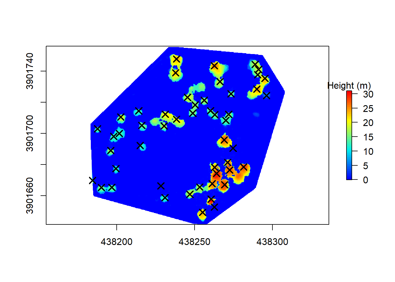
Adam Belmonte
Applied Scientist
I am a remote sensing and data scientist focused on natural resource management.